Temporal P/NP Theory: Mathematical Formalization

1. Core Definitions

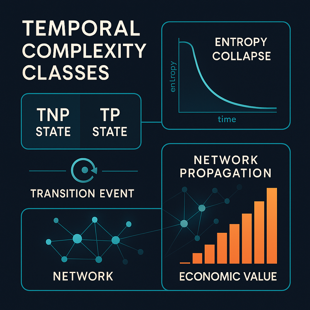
1.1 Temporal Complexity Classes

Let Π be a computational problem with solution space S.

Definition 1.1 (Temporal NP State): A problem Π is in temporal NP state at time t, denoted Π ∈ TNP(t), if:

• No algorithmic solution exists at time t
• Verification time V(s) << Discovery time D(s) for any solution s ∈ S
• System time cannot compress the discovery process

Definition 1.2 (Temporal P State): A problem Π is in temporal P state at time t, denoted Π ∈ TP(t), if:

• An algorithmic solution A exists at time t
• Execution time E(A) ≈ V(s) for solutions s
• System time can optimize the known algorithm

1.2 The Transition Function

Definition 1.3 (P/NP Transition Event): The transition τ(Π) occurs at time t* when:

τ(Π) = min{t : ∃h ∈ H, h discovers algorithmic solution A for Π}

Where H is the set of human problem-solvers.

2. Thermodynamic Formulation

2.1 Entropy Evolution

Definition 2.1 (Problem Entropy): The entropy of problem Π at time t:

S(Π,t) = -k ∑_{s∈S} p(s,t) ln p(s,t)

Where:

• p(s,t) = probability of solution s being explored at time t
• k = information constant

Theorem 2.1 (Entropy Collapse): At transition τ(Π):

lim_{t→τ⁺} S(Π,t) << lim_{t→τ⁻} S(Π,t)

The entropy collapses as the solution space crystallizes into an algorithm.

2.2 Time Violence Quantification

Definition 2.2 (Time Violence): The temporal inefficiency for problem Π:

TV(Π,t) = {
    ∫[H(τ) - S(τ)]² dτ,  if Π ∈ TNP(t)
    α·[t - τ(Π)],         if Π ∈ TP(t)
}

Where:

• H(τ) = human temporal position
• S(τ) = system temporal position
• α = decay constant for optimization value

3. Network Propagation Dynamics

3.1 Discovery-Verification Coupling

Definition 3.1 (Network Invariant Speed): Following the harmonic mean principle:

C_N = (v_d · v_v)/(v_d + v_v)

Where:

• v_d = discovery rate (problems/time transitioning from TNP to TP)
• v_v = verification/implementation rate

Theorem 3.1 (Propagation Bound): The rate of P/NP transitions in a network is bounded by:

dN_P/dt ≤ C_N · N_{TNP}

Where N_P and N_{TNP} are the number of problems in each state.

3.2 Sub-Universe Exploration

Definition 3.2 (Parallel Exploration): Given n sub-universes {U₁, U₂, ..., Uₙ} exploring problem Π:

P(τ(Π) ≤ t) = 1 - ∏ᵢ₌₁ⁿ [1 - Pᵢ(t)]

Where Pᵢ(t) is the probability that universe i solves Π by time t.

4. Economic Value Formulation

4.1 First-Solver Advantage

Definition 4.1 (Transition Value): The economic value of achieving transition τ(Π):

V(τ) = ∫_{τ}^{τ+Δt} [R(t) · e^{-λ(t-τ)}] dt

Where:

• R(t) = revenue rate from problem solution
• λ = decay rate as systems catch up
• Δt = exploitation window

Theorem 4.1 (Temporal Monopoly): The first-solver maintains advantage for duration:

Δt ≈ (1/v_v) · ln(S(Π,τ⁻)/S_min)

Proportional to the log of entropy reduction achieved.

4.2 Innovation Chain Dynamics

Definition 4.2 (Problem Generation Rate): New TNP problems emerge at rate:

g(t) = β · N_P(t) · ⟨C⟩

Where:

• β = innovation constant
• N_P(t) = number of solved problems
• ⟨C⟩ = average problem complexity

5. Temporal Lag Formalization

5.1 Human-System Gap

Definition 5.1 (Temporal Gap): The lag between human and system time:

Δ(t) = ∫₀ᵗ [g(τ) - C_N] dτ

Theorem 5.1 (Divergence Condition): The system diverges when:

g(t) > C_N

Leading to unbounded growth in unsolved problems.

5.2 Complexity Inflation

Definition 5.2 (Complexity Inflation Rate): The rate at which problem complexity grows:

dC/dt = γ · [g(t) - C_N]⁺ · C

Where [x]⁺ = max(0,x) and γ is the inflation constant.

6. Optimization Strategies

6.1 Temporal Field Enhancement

Strategy 6.1 (Discovery Acceleration): Maximize individual discovery rates through:

v_d^* = v_d⁰ · (1 + ∑ᵢ wᵢ · Iᵢ)

Where:

• v_d⁰ = baseline discovery rate
• Iᵢ = information from temporal field i
• wᵢ = trust weight for source i

6.2 Network Architecture

Strategy 6.2 (Tripartite Optimization): For the Product-Media-Education trinity:

Efficiency = (v_p · v_m · v_e)^(1/3) / [(1/v_p + 1/v_m + 1/v_e)/3]

Maximized when v_p = v_m = v_e (balanced system).

7. Fundamental Theorems

7.1 The Temporal P/NP Theorem

Theorem 7.1 (Main Result): In any network with finite C_N and growing complexity:

1. All problems begin in TNP state
2. Human discovery is necessary for TNP → TP transition
3. System optimization always lags by Δt > 0
4. Value accrues disproportionately to first solvers

Proof Sketch:

• By construction, no algorithm exists before discovery
• Discovery requires exploration of solution space (human time)
• Implementation requires codification (system time)
• Temporal ordering ensures discoverer advantage □

7.2 The Entropy-Value Correspondence

Theorem 7.2 (Entropy-Value): The economic value of a transition is proportional to entropy reduction:

V(τ) ∝ S(Π,τ⁻) - S(Π,τ⁺)

Implication: Highest value comes from solving the most disordered problems.

8. Conclusions

This formalization reveals:

1. P/NP transitions are irreversible temporal events
2. Human time necessarily leads system time
3. Economic value concentrates at transition moments
4. Networks have fundamental speed limits C_N
5. Complexity inflation is inevitable without active management

The mathematics suggest that rather than fighting this temporal structure, we should design systems that:

• Accelerate human discovery (increase v_d)
• Streamline verification (increase v_v)
• Distribute transition rewards fairly
• Manage complexity inflation actively

This creates a new lens for understanding innovation, computation, and economic value in the age of accelerating information.